PDP - Amdahl's law, Gustafson's law, and Isoefficiency functions

First 5 minutes of hell

Scalability = the property of the parallel algorithm to keep the parallel optimality if both $p$ and $n$ grow or shrink.

Amdahl’s Law for saturation of parallelizability

• $S(n,p)=\frac{T_A(n)}{f_s\cdot T_A(n)+\frac{1-f_s}{p}\cdot T_A(n)}=\frac{1}{f_s+\frac{1-f_s}{p}}\le \frac{1}{f_s}$
  • at each sequential algorithm $T_A(n)$, there is an inherently sequential fraction (executed only on 1 thread - I/O operations, initialization etc.) $f_s$ and the the parallelizable $1-f_s$ part
  • the sequential part is not parallelizable, so it bounds the speedup (at some point, adding more processors does not increase the speedup anymore)
  • essentially saying that if we have fixed problem size $n$, there is only a limited amount of parallelism to do (it cannot be scaled to the infinity)

Gustavson’s Law

• Setup: split the parallel execution time into t_seq (sequential part) and t_par(n,p) (parallel part, executed on p processors)
  • $S(n,p)=\frac{t_{\text{seq}}+p\cdot t_{\text{par}}(n,p)}{t_{\text{seq}}+t_{\text{par}}(n,p)}$
  • let $f_s$ be the fraction of the parallel execution time spent on the sequential part: $f_s=\frac{t_{\text{seq}}}{t_{\text{seq}}+t_{\text{par}}(n,p)}$
  • then the speedup simplifies to: $S(n,p)=f_s+p\cdot (1-f_s)=p-f_s\cdot (p-1)$
• limit (assuming $t_{\text{par}}$ grows with $n$ while $t_{\text{seq}}$ stays fixed): ${\lim }_{n\to \infty }S(n,p)=p$
  • Gustavson assumes that as we get more processors, we scale the problem size (rather than keeping it fixed), under this assumption, linear speedup is achievable

Isoefficiency functions

• when preserving the efficiency, we need to define the best ratio of processors $p$ and the problem size $n$, and the isoefficiency functions define the upper and lower bound of this relationship
• for a given constant efficiency $0<E_0<1$:
  • the minimum n needed for a given p: $\forall n_p=\Omega ({\psi }_1(p)):E(n_p,p)\ge E_0$
    • Gustavson essentially says that if the problem size $n$ grows according to the $p$, the efficiency will be sufficiently good
  • the maximum p allowed for a given n: $\forall p_n=O({\psi }_2(n)):E(n,p_n)\ge E_0$
    • = for a fixed size $n$, how many processors can I use while still maintaining the efficiency at least $E_0$
    • it is the largest function, so any more processors beyond this and the efficiency drops below $E_0$ (we will be wasting them)
      • this is what the Amdahl’s Law is saying, if I use more processors, I “saturate” the parallelism and adding more processors won’t help
      • the ${\psi }_2(n)$ is the saturation point, where I am hitting the $\frac{1}{f_s}$ ceiling

Parallel scalability

• definition: scalability is the property of a parallel algorithm to keep the parallel optimality if both $p$ and $n$ grow or shrink
  • the scalability expresses that larger problems can be solved in the same time as smaller problems if sufficient $p$ is utilized
  • it’s not always about having a maximum number of processing units $p$ available
    • it’s the scalability issue, we have to scale $p$ with $n$ to keep all cores busy all the time
• 
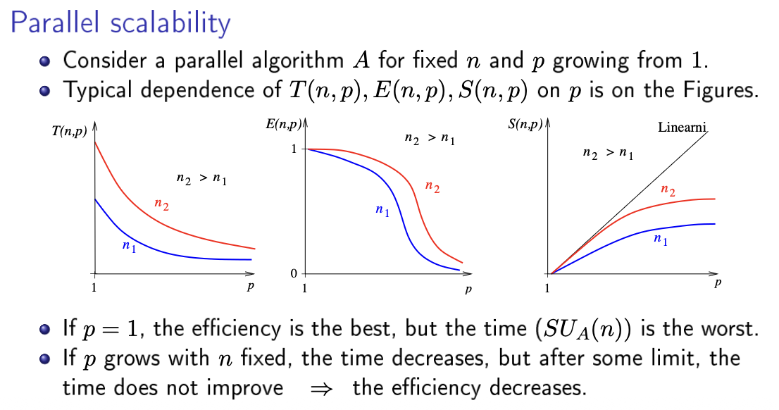
  • T - time, E - efficiency, S - speedup
• there are two types of scalability:
  • strong scalability: measures the capability of a parallel algorithm for fixed $n$ to achieve linear speedup with increasing p (Amdahl’s law puts strong limits to this)
    • alternatively: strong scalability is the measure of efficiency decrease if $p$ increases while $n$ is fixed
  • weak scalability: defines how the parallel time varies with $p$ for fixed $n/p$
    • alternatively: weak scalability is the measure of growth of $n$ such that a fixed efficiency is preserved when $p$ increases

Amdahl’s Law

• each sequential calculation has some part of it inherently sequential, call it $f_s$
  • the remaining part of $1-f_s$ could be parallelized
  • we assume the perfect parallelization without any overhead
• derivation: let $T(1)=T_s+T_p$ be the sequential time, with $f_s=T_s/T(1)$
  • under perfect parallelization the parallel time $T(p)$ is $T(p)=T_s+T_p/p=f_s\cdot T(1)+(1-f_s)\cdot T(1)/p$
  • dividing $T(1)$ by $T(p)$ yields the formula below
• the formula ($n$ is fixed, $p$ varies): $S(n,p)=\frac{T_A(n)}{f_s\cdot T_A(n)+\frac{1-f_s}{p}\cdot T_A(n)}=\frac{1}{f_s+\frac{1-f_s}{p}}\le \frac{1}{f_s}$- the law:
  • the parallel speedup $S(n,p)$ will always be bounded by $\frac{1}{f_s}$ no matter how many threads are used
  • it measures the parallel algorithm efficiency decrease if $p$ is increasing while $n$ is fixed
    • that every added processor has more marginal benefit
    • after a certain value of $p$, adding new processors does not make sense, there is not enough parallel work to do (see the above plots)
      • that is called the saturation limit
  • it basically says that a fixed size problem provides a limited amount of parallellism (there is a limit of a reasonable number of parallel threads to execute it)
• examples:
  • if $f_s=10\%$, the speedup will be $S(n,p)\le 10$ for any $p$
    • no matter how many processors in parallel I use, the speedup will be at most 10 times faster (because the non-parallelizable 10 % of sequential time will be a bottleneck)
  • if $f_s=20\%$, the speedup $S(n,p)\le 5$ for any $p$

Gustafson’s Law

• weak scalability: if we scale $n$ and $p$ linearly together, a constant efficiency can be maintained
  • and thus the linear speedup and optimal cost
  • meaning, if we add more computing units $p$, we should also scale up the problem size $n$
  • it measures the $n$ growth when we preserve the efficiency while increasing $p$
• the non-parallelizable sequential portion stays constant (I/O operations, initialization…), so as we add processors $p$ and proportionally grow the problem $n$, the parallel portion scales linearly, hence overall speedup is linear in p
• the formula (here $f_s$ is the sequential fraction of the parallel execution time on the scaled problem, not of the serial time): $S(n,p)=f_s+(1-f_s)\cdot p=p-f_s(p-1)$
• reconciliation with Amdahl: the two laws are not contradictory, they answer different questions
  • Amdahl fixes $n$ and asks how speedup behaves with $p$ - strong scaling, pessimistic
  • Gustafson fixes time-per-processor and lets $n$ grow with $p$ - weak scaling, optimistic
  • the apparent disagreement comes from where $f_s$ is measured: Amdahl on the serial execution, Gustafson on the scaled parallel execution

Isoefficiency functions

• when preserving the efficiency of the parallel algorithm, isoefficiency functions define the lowerbound and upperbound of the $n$ and $p$ relationship
• we can define some fixed efficiency that we want to achieve, e.g. 0.2 (20 %):
  • the isoefficiency functions specify:
    • the minimum n needed for a given p: $\forall n_p=\Omega ({\psi }_1(p)):E(n_p,p)\ge E_0$
    • the maximum p allowed for a given n: $\forall p_n=O({\psi }_2(n)):E(n,p_n)\ge E_0$
  • to maintain the given efficiency guarantee
• we ask: “what minimum efficiency do I want to guarantee?”
  • and with isoefficiency functions, I can calculate the correct scaling of n and p to maintain this efficiency (when I have to option to remove/add computing units and increase/decrease the problem size)
• the isoefficiency is the property of the algorithm, not of the problem
  • different algorithms of the same problem can have differernt isoefficiency values

Potential exam questions

1. Derive Amdahl’s law from $T(1)=T_s+T_p$ assuming perfect parallelization of the parallelizable part.
2. State Amdahl’s formula and compute the asymptotic speedup limit for $f_s=5\%$.
3. What is the saturation limit and why does adding more processors beyond it not help?
4. State Gustafson’s formula. How is $f_s$ defined differently than in Amdahl’s law?
5. Are Amdahl’s law and Gustafson’s law contradictory? Explain.
6. Define strong scalability and weak scalability. Which law is associated with which?
7. Define efficiency in terms of sequential work $T_s$ and parallel overhead $T_o$, and explain how this leads to the notion of isoefficiency.
8. What does it mean for an algorithm to have isoefficiency function $\Theta (p\log p)$? Is this better or worse than $\Theta (p^2)$?
9. Derive the isoefficiency function of parallel reduction on $p$ processors.
10. Explain why isoefficiency is a property of the algorithm, not of the problem. Give an intuitive argument.